Find the Constant a Such That the Function is Continuous on the Entire Real Line Webassign
| | SECTION 3.2 | Graphs of Functions; Piecewise-Defined Functions; Increasing and Decreasing Functions; Average Rate of Change |
|
| ||||||||||||||||||||||||||||||||||||||||||||||||||
 �
�
Recognizing and Classifying Functions
3.2.1.1�Common Functions
Point-plotting techniques were introduced in Section 2.2, and we noted there that we would explore some more efficient ways of graphing functions in Chapter 3. The nine main functions you will read about in this section will constitute a "library" of functions that you should commit to memory. We will draw on this library of functions in the next section when graphing transformations are discussed. Several of these functions have been shown previously in this chapter, but now we will classify them specifically by name and identify properties that each function exhibits.
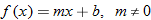
In Section 2.3, we discussed equations and graphs of lines. All lines (with the exception of vertical lines) pass the vertical line test, and hence are classified as functions. Instead of the traditional notation of a line,  , we use function notation and classify a function whose graph is a line as a linear function.
The domain of a linear function 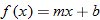 is the set of all real numbers
  . The graph of this function has slope
  and
and  .
.
One special case of the linear function is the constant function  .
.
| | |
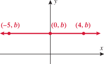
The graph of a constant function  is a horizontal line. The
  corresponds to the point
  . The domain of a constant function is the set of all real numbers . The range, however, is a single value
  . In other words, all
  correspond to a single
  .
.
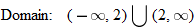
| Points that lie on the graph of a constant function | Domain: |
| | |
| | |
| | |
| | |
| | |
| | |
| | � |
 or
or 


Another specific example of a linear function is the function having a slope of one  and a of zero
  . This special case is called the identity function.

A function that squares the input is called the square function.

The graph of the square function is called a parabola and will be discussed in further detail in Chapters 4 and 8. The domain of the square function is the set of all real numbers . Because squaring a real number always yields a positive number or zero, the range of the square function is the set of all nonnegative numbers. Note that the intercept is the origin and the square function is symmetric about the  . This graph is contained in quadrants I and II.
A function that cubes the input is called the cube function.

The domain of the cube function is the set of all real numbers . Because cubing a negative number yields a negative number, cubing a positive number yields a positive number, and cubing 0 yields 0, the range of the cube function is also the set of all real numbers . Note that the only intercept is the origin and the cube function is symmetric about the origin. This graph extends only into quadrants I and III.
The next two functions are counterparts of the previous two functions: square root and cube root. When a function takes the square root of the input or the cube root of the input, the function is called the square root function or the cube root function, respectively.
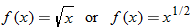
In Section 3.1, we found the domain to be  . The output of the function will be all real numbers greater than or equal to zero. Therefore, the range of the square root function is . The graph of this function will be contained in quadrant I.
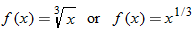
In Section 3.1, we stated the domain of the cube root function to be  . We see by the graph that the range is also . This graph is contained in quadrants I and III and passes through the origin. This function is symmetric about the origin.
In Section 1.7, you read about absolute value equations and inequalities. Now we shift our focus to the graph of the absolute value function.

Some points that are on the graph of the absolute value function are  ,
,  , and
, and  . The domain of the absolute value function is the set of all real numbers , yet the range is the set of nonnegative real numbers. The graph of this function is symmetric with respect to the
  and is contained in quadrants I and II.
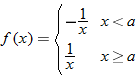
A function whose output is the reciprocal of its input is called the reciprocal function.
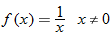
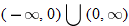
The only restriction on the domain of the reciprocal function is that  . Therefore, we say the domain is the set of all real numbers excluding zero. The graph of the reciprocal function illustrates that its range is also the set of all real numbers except zero. Note that the reciprocal function is symmetric with respect to the origin and is contained in quadrants I and III.
3.2.1.2�Even and Odd Functions
Of the nine functions discussed above, several have similar properties of symmetry. The constant function, square function, and absolute value function are all symmetric with respect to the . The identity function, cube function, cube root function, and reciprocal function are all symmetric with respect to the origin. The term even is used to describe functions that are symmetric with respect to the , or vertical axis, and the term odd is used to describe functions that are symmetric with respect to the origin. Recall from Section 2.2 that symmetry can be determined both graphically and algebraically. The box below summarizes the graphic and algebraic characteristics of even and odd functions.
| EVEN AND ODD FUNCTIONS |
| Function | Symmetric with Respect to | On Replacing |
|---|---|---|
| Even | | |
| Odd | origin | |
The algebraic method for determining symmetry with respect to the , or vertical axis, is to substitute  for
for  . If the result is an equivalent equation, the function is symmetric with respect to the . Some examples of even functions are , ,
  ; and .
| | |

In any of these equations, if is substituted for , the result is the same; that is, 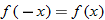 . Also note that, with the exception of the absolute value function, these examples are all even-degree polynomial equations. All constant functions are degree zero and are even functions.
The algebraic method for determining symmetry with respect to the origin is to substitute for . If the result is the negative of the original function, that is, if 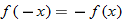 , then the function is symmetric with respect to the origin and, hence, classified as an odd function. Examples of odd functions are , ,
  , and
, and  . In any of these functions, if is substituted for , the result is the negative of the original function. Note that with the exception of the cube root function, these equations are odd-degree polynomials.
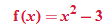
Be careful, though, because functions that are combinations of even- and odd-degree polynomials can turn out to be neither even nor odd, as we will see in Example 1.
| �EXAMPLE� 1� | Determining Whether a Function Is Even, Odd, or Neither |
Determine whether the functions are even, odd, or neither.
| | |
Solution
| |
| ||||||||||||||||||||||||||||||||||||
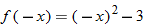
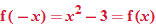
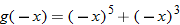
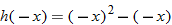
 , we say that
 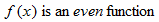 .
.

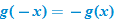 , we say that
 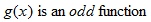 .
.
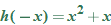
 therefore the function
  is
is 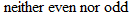 .
.In parts (a), (b), and (c), we classified these functions as either even, odd, or neither, using the algebraic test. Look back at them now and reflect on whether these classifications agree with your intuition. In part (a), we combined two functions: the square function and the constant function. Both of these functions are even, and adding even functions yields another even function. In part (b), we combined two odd functions: the fifth-power function and the cube function. Both of these functions are odd, and adding two odd functions yields another odd function. In part (c), we combined two functions: the square function and the identity function. The square function is even, and the identity function is odd. In this part, combining an even function with an odd function yields a function that is neither even nor odd and, hence, has no symmetry with respect to the vertical axis or the origin.
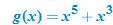
| Classify the functions as even, odd, or neither.
|


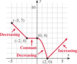
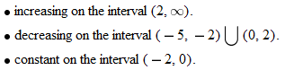
Increasing and Decreasing Functions
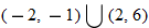
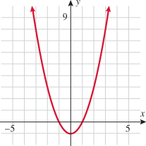
When specifying a function as increasing, decreasing, or constant, the intervals are classified according to the  .
.
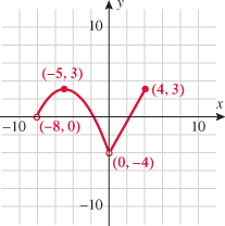
| | |

For instance, in this graph, we say the function is increasing when is between  and
and  and again when
  is between
  and
and  . The graph is classified as decreasing when is less than
  and again when is between 0 and 2 and again when is greater than 6. The graph is classified as constant when is between
  and 0. In interval notation, this is summarized as
| Decreasing | Increasing | Constant |
|---|---|---|
| | | |

An algebraic test for determining whether a function is increasing, decreasing, or constant is to compare the value  of the function for particular points in the intervals.
| INCREASING, DECREASING, AND CONSTANT FUNCTIONS |
In addition to classifying a function as increasing, decreasing, or constant, we can also determine the domain and range of a function by inspecting its graph from left to right:
| |
| ||||||||||||||||||||
 (from bottom to top) that the graph of the function corresponds to.
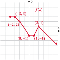
| �EXAMPLE� 2� | Finding Intervals When a Function Is Increasing or Decreasing |
Given the graph of a function:
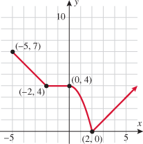
| (a)�� | State the domain and range of the function. |
| (b)�� | Find the intervals when the function is increasing, decreasing, or constant. |
Solution
| |
| ||||||||

 .
. 
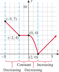
 is included in the domain of the function but not in the interval where the function is classified as decreasing.
Average Rate of Change
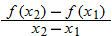
How do we know how much a function is increasing or decreasing? For example, is the price of a stock slightly increasing or is it doubling every week? One way we determine how much a function is increasing or decreasing is by calculating its average rate of change.
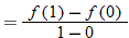
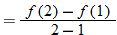
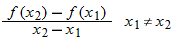
Note that the slope of the secant line is given by  , and recall that the slope of a line is the rate of change of that line. The slope of the secant line is used to represent the average rate of change of the function.
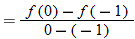
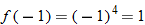
| �EXAMPLE� 3� | Average Rate of Change |
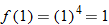
Find the average rate of change of from:
| (a)�� | |
| (b)�� | |
| (c)�� | |
Solution
| |
| ||||||||||||||||||||||||||||||||||||
 and
and  .
.
 and
and  .
.


 and
and  .
.
 .
.

 and
and  .
.
 and
and 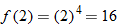 .
.

| | Graphical Interpretation: Slope of the Secant Line
| ||||||||||||
| Find the average rate of change of |
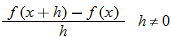
The average rate of change can also be written in terms of the difference quotient.
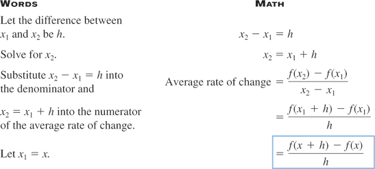
When written in this form, the average rate of change is called the difference quotient.
| DEFINITION� | Difference Quotient |
The expression 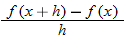 , where
  , is called the difference quotient.
The difference quotient is more meaningful when  is small. In calculus the difference quotient is used to define a derivative.
| EXAMPLE� 4� | Calculating the Difference Quotient |
Calculate the difference quotient for the function 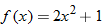 .
.
| Calculate the difference quotient for the function |
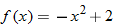 .
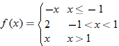
.Piecewise-Defined Functions
Most of the functions that we have seen in this text are functions defined by polynomials. Sometimes the need arises to define functions in terms of pieces. For example, most plumbers charge a flat fee for a house call and then an additional hourly rate for the job. For instance, if a particular plumber charges  to drive out to your house and work for 1 hour and then an additional
  an hour for every additional hour he or she works on your job, we would define this function in pieces. If we let be the number of hours worked, then the charge is defined as
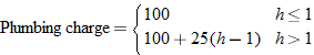
If we were to graph this function, we would see that there is 1 hour that is constant and after that the function continually increases.
The next example is a piecewise-defined function given in terms of functions in our "library of functions." Because the function is defined in terms of pieces of other functions, we draw the graph of each individual function, and then for each function, darken the piece corresponding to its part of the domain. This is like the procedure above for the absolute value function.
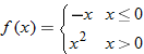
| EXAMPLE� 5� | Graphing Piecewise-Defined Functions |
Graph the piecewise-defined function, and state the domain, range, and intervals when the function is increasing, decreasing, or constant.
Solution
| Graph each of the functions on the same plane. | |
| Square function: | |
| Constant function: | |
| Identity function: | � |
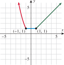
The points to focus on in particular are the where the pieces change over—that is, and  .
.
Let's now investigate each piece. When  , this function is defined by the square function,
  , so darken that particular function to the left of . When
  , the function is defined by the constant function,
  , so darken that particular function between the values of and 1. When
  , the function is defined by the identity function,
  , so darken that function to the right of . Erase everything that is not darkened, and the resulting graph of the piecewise-defined function is given on the right. This function is defined for all real values of , so the domain of this function is the set of all real numbers. The values that this function yields in the vertical direction are all real numbers greater than or equal to 1. Hence, the range of this function is
  . The intervals of increasing, decreasing, and constant are as follows:
The term continuous implies that there are no holes or jumps and that the graph can be drawn without picking up your pencil. A function that does have holes or jumps and cannot be drawn in one motion without picking up your pencil is classified as discontinuous, and the points where the holes or jumps occur are called points of discontinuity.
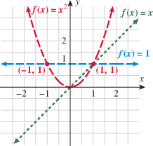
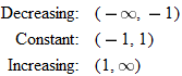
The previous example illustrates a continuous piecewise-defined function. At the junction, the square function and constant function both pass through the point . At the junction, the constant function and the identity function both pass through the point . Since the graph of this piecewise-defined function has no holes or jumps, we classify it as a continuous function.
The next example illustrates a discontinuous piecewise-defined function.
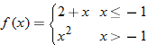
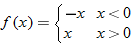
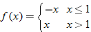
| �EXAMPLE� 6� | Graphing a Discontinuous Piecewise-Defined Function |
Graph the piecewise-defined function, and state the intervals where the function is increasing, decreasing, or constant, along with the domain and range.
Solution
| Graph these functions on the same plane. | |
| Linear function: | |
| Identity function: | |
| Constant function: |


Darken the piecewise-defined function on the graph. For all values less than zero  the function is defined by the linear function . Note the use of an open circle, indicating up to but not including
  . For values
  , the function is defined by the identity function .
The circle is filled in at the left endpoint, . An open circle is used at . For all values greater than 2,  , the function is defined by the constant function . Because this interval does not include the point , an open circle is used.
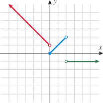
At what intervals is the function increasing, decreasing, or constant? Remember that the intervals correspond to the  .
.
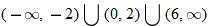
| Decreasing: | Increasing: | Constant: |


The function is defined for all values of except .
The output of this function (vertical direction) takes on the  and the additional single value
  .
.

We mentioned earlier that a discontinuous function has a graph that exhibits holes or jumps. In this example, the point corresponds to a jump, because you would have to pick up your pencil to continue drawing the graph. The point corresponds to both a hole and a jump. The hole indicates that the function is not defined at that point, and there is still a jump because the identity function and the constant function do not meet at the same  at .
at .
| Graph the piecewise-defined function, and state the intervals where the function is increasing, decreasing, or constant, along with the domain and range. |
Piecewise-defined functions whose "pieces" are constants are called step functions. The reason for this name is that the graph of a step function looks like steps of a staircase. A common step function used in engineering is the Heaviside step function (also called the unit step function):
This function is used in signal processing to represent a signal that turns on at some time and stays on indefinitely.
A common step function used in business applications is the greatest integer function.
| GREATEST INTEGER FUNCTION |
 .
.
| | 1.0 | 1.3 | 1.5 | 1.7 | 1.9 | 2.0 |
| | 1 | 1 | 1 | 1 | 1 | 2 |

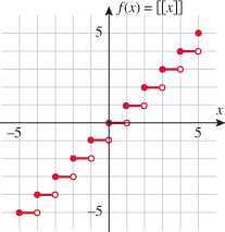
| | |
| ||||||||||||||||||||||||||||||||||||||||||||||||||||||||||||||||||||||||||||||||||||||||||||||||||
| ||||||||||||||||||||||||||||||||||||||||||||||||||||||||||||||||||||||||||||||||||||||||||||||||||

 )
)
 or
or 


| | SECTION 3.2 | EXERCISES |
In Exercises 1-24, determine whether the function is even, odd, or neither.
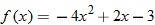
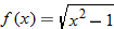
| 2.�� | |

| 4.�� | |
| 6.�� | |
| 8.�� | |
| 10.�� | |
| 12.�� | |
| 14.�� | |

| 16.�� | |

| 18.�� | |

| 20.�� | |
| 22.�� | |

| 24.�� | |
| 26.�� | |
| 28.�� | |
| 30.�� | |
| 32.�� | |
| 34.�� | |
| 36.�� | |
In Exercises 37-44, find the difference quotient for each function.
| 38.�� | |
| 40.�� | |
| 42.�� | |
| 44.�� | |
In Exercises 45-52, find the average rate of change of the function from to  .
.
| 46.�� | |
| 48.�� | |

| 50.�� | |

| 52.�� | |
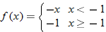
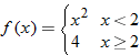
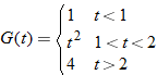
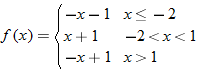
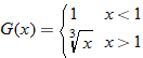
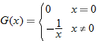
In Exercises 53-78, graph the piecewise-defined functions. State the domain and range in interval notation. Determine the intervals where the function is increasing, decreasing, or constant.
| 54.�� | |
| 56.�� | |
| 58.�� | |
| 60.�� | |
| 62.�� | |
| 64.�� | |
| 66.�� | |
| 68.�� | |
| 70.�� | |
| 72.�� | |
| 74.�� | |
| 76.�� | |
| 78.�� | |
For Exercises 79 and 80, refer to the following:
A manufacturer determines that his profit and cost functions over one year are represented by the following graphs.
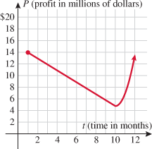
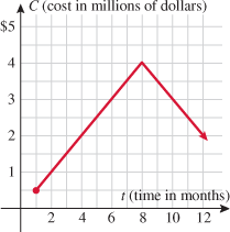
| 79.�� | Business. Find the intervals on which profit is increasing, decreasing, and constant. |

| 80.�� | Business. Find the intervals on which cost is increasing, decreasing, and constant. |
| 81.�� | Budget: Costs. |
| 83.�� | Budget: Costs. |
| 84.�� | Phone Cost: Long-Distance Calling. |
| 85.�� | Event Planning. |
| 87.�� | Sales. |
| 89.�� | Profit. |
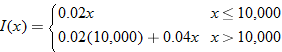
| 91.�� | Postage Rates. The following table corresponds to first-class postage rates for the U.S. Postal Service. Write a piecewise-defined function in terms of the greatest integer function that models this cost of mailing flat envelopes first class.
Observe that Using the greatest integer function, we have |
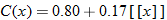 where
where 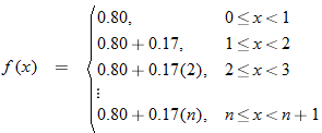
 .
.| 92.�� | Postage Rates. The following table corresponds to first-class postage rates for the U.S. Postal Service. Write a piecewise-defined function in terms of the greatest integer function that models this cost of mailing parcels first class.
A square wave is a waveform used in electronic circuit testing and signal processing. A square wave alternates regularly and instantaneously between two levels. |
| 93.�� | Electronics: Signals. Write a step function |
 that represents the following square wave.
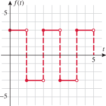
| 94.�� | Electronics: Signals. |
For Exercises 95 and 96, refer to the following table:
| Global Carbon Emissions from Fossil Fuel Burning | ||||||||||||
|
| 95.�� | Climate Change: Global Warming. What is the average rate of change in global carbon emissions from fossil fuel burning from
|
| 96.�� | Climate Change: Global Warming. What is the average rate of change in global carbon emissions from fossil fuel burning from |
For Exercises 97 and 98, use the following information:
The height (in feet) of a falling object with an initial velocity of  per second launched straight upward from the ground is given by
  , where
  is time (in seconds).
| 97.�� | Falling Objects. What is the average rate of change of the height as a function of time from |
 ?
?| 98.�� | Falling Objects. What is the average rate of change of the height as a function of time from |
 ?
?For Exercises 99 and 100, refer to the following:
An analysis of sales indicates that demand for a product during a calendar year (no leap year) is modeled by
where  is demand in thousands of units and is the day of the year and
  represents January 1.
| 99.�� | Economics. Find the average rate of change of the demand of the product over the first quarter. |
| 100.�� | Economics. Find the average rate of change of the demand of the product over the fourth quarter. |
In Exercises 101-104, explain the mistake that is made.
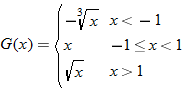
| 101.�� | Graph the piecewise-defined function. State the domain and range. Solution: This is incorrect. What mistake was made? |
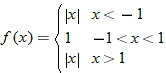
| 102.�� | Graph the piecewise-defined function. State the domain and range. Solution: Domain: This is incorrect. What mistake was made? |

| 103.�� | The cost of airport Internet access is Solution: This is incorrect. What mistake was made? |
 for the first 30 minutes and
  per minute for each additional minute. Write a function describing the cost of the service as a function of minutes used online.
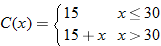
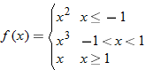
| 104.�� | Solution: This is incorrect. What mistake was made? |
In Exercises 105-108, determine whether each statement is true or false.
| 105.�� | The identity function is a special case of the linear function. |
| 106.�� | The constant function is a special case of the linear function. |
| 107.�� | If an odd function has an interval where the function is increasing, then it also has to have an interval where the function is decreasing. |
| 108.�� | If an even function has an interval where the function is increasing, then it also has to have an interval where the function is decreasing. |
| 110.�� | |
| 111.�� | |
| 113.�� | |
| 114.�� | Plot the function |
 . What function is this?
| 115.�� | Graph the function |
 using a graphing utility. State the domain and range.
| 116.�� | Graph the function |
 using a graphing utility. State the domain and range.
Source: https://www.webassign.net/ebooks/youngat3demo/young9780470648018/c03/young9780470648018c03_3_0_body.htm
0 Response to "Find the Constant a Such That the Function is Continuous on the Entire Real Line Webassign"
Post a Comment